Neo4j & DGL — a seamless integration
In this article we will illustrate how to integrate a Graph Attention Network model using the Deep Graph Library into the Neo4j workflow and deploying the Neo4j Python driver.
This blog post was co-authored with Clair Sullivan and Mark Needham
Introduction
The release of the Neo4j GDS library version 1.5, and the build-in machine learning models, has now given the Data Scientist that needs to perform a machine learning task on any graph in Neo4j two possible routes to a solution.
If time is of the essence and a supported and tested model that works natively is needed, then a simple function call to the GDS library will get the job done. If, however, more flexibility is needed or there are some data constraints then the Data Scientist can deploy external machine learning libraries, in conjunction with the Neo4j Python driver.
In these series of articles we will illustrate how different external Machine Learning libraries can be used to complement the existing Neo4j Graph Data Science (GDS) functionality.
For this article we have used the Deep Graph Library (DGL) package with TensorFlow as backend and have constructed a Colab notebook with the entire code using the Cora dataset, which can be found here.
Graph Neural Networks
By way of background, we briefly describe Graph Neural Networks (GNNs), which in its broadest sense can be defined as a class of neural network models suitable for processing graph-structured data. As such, and again in its broadest sense, learning on graphs (i.e. Graph Representation Learning) can be divided into two classes of learning problems; unsupervised and supervised learning (incl. semi-supervised). Unsupervised learning aims at learning low-dimensional Euclidean representations that capture the structure of the input graph, these are generally known as embedding algorithms, and an example of which is the Node2Vec algorithm which can be found in the Neo4j GDS library. The second class of learning tasks also learns an embedding but with the goal of performing some downstream prediction such as node or graph classification or link prediction. Whereas the inputs for the unsupervised learning are typically the entire graph, for the supervised task the inputs are node features and possibly edge features and in addition, the graph structure (all or usually partly) can also be used in training. The general framework for the supervised GNN task is a ‘message passing’ framework that aims to encompass the different types of GNNs. Recent surveys organize the different GNNs in a taxonomy of around 5 GNN architectures, ranging from Recurrent GNNs, Graph Convolutional NNs to Graph Attention Networks etc.
Now, the Data Scientist may want to exploit these different architectures since she/he may face issues of having a limited amount of labeled data and therefore can only deploy semi-supervised models, or may want to gain additional insights from the most important features etc. Hence, in those circumstances, the Data Scientist will want to build their own customized model to make node classifications or other downstream applications.
Thanks to the Neo4j Python driver any of the GNN packages are available to perform graph machine learning tasks on a Neo4j graph. Indeed, in the past few years, a whole smorgasbord of libraries and tools have been developed, by a recent count the number of open source projects on Graph Neural Networks has reached almost 100!
Deep Graph Library
The DGL package is one of the most extensive libraries consisting of the core building blocks to create graphs, several message passing functions, as well as entire Graph Neural Network models, all ready to go. Another advantage of the DGL library is that it works with the most frequently used backend platforms such as TensorFlow, Pytorch, and MXNet. Finally, DGL comes with a data API that provides access to some of the benchmark datasets, one of which is the Cora citation graph, which is pretty much the equivalent of MNIST in graph land…
Graph Attention Network
One such GNN that a Data Scientist may want to use could be a Graph Attention Network. This is a semi-supervised learning model that only needs a limited number of known labels, in addition to the node features, to train the model. It does this by computing the hidden representations of each node in the graph by giving “attention” to the neighbors of that specific node. That is, it applies an “attention-based architecture” to perform node classification.
The Theory
Before we jump into the experiment, we’ll first explain the GNN model we are deploying. Graph ATtention Networks (abbreviated ‘GAT’, such as not to confuse with, Generative Adversarial Networks) were introduced in 2018 by Velickovic et al. as an improvement to existing Graph Convolutional Neural Networks. As the name suggests, the core idea of GATs is to apply an ‘attention mechanism’ based architecture.
Attention mechanisms revolutionized neural machine translation, and NLP in general, and have become the de facto’ norm in many sequence-based models. An attention mechanism can broadly be divided into two main categories: ‘general attention’ which quantifies the independence between input and output elements, and ‘self-attention’ which manages and quantifies the independence within input elements. In the GAT model, the role of the attention mechanism is “to compute the hidden representations of each node in the graph by attending over its neighbors” following a self-attention strategy.
We will briefly describe the key steps and components of a single ‘graph attention layer’ and refer the interested reader to the paper for a more detailed and mathematical explanation.
The narrative of the model can be summarized in 5 steps:

- The first step is to define the set of node features that provide the input to the model. As we will see, in our example, these are the feature vectors obtained by embedding the text of each document in a 0/1 “bag-of-words” vector of length 1433.
- As a second step, we apply a linear transformation to each feature vector using a shared weight matrix of learnable parameters.
- The third step involves performing the self-attention by computing the attention coefficients as follows: we concatenate two linearly transformed node features (linearly transformed in step 1), of the source and destination node, and apply the attention mechanism. This mechanism is nothing more than applying a LeakyReLu nonlinear activation function to the dot product of a learnable weight vector (let’s call it a) with the concatenated node features. As such, the attention mechanism can be viewed as a single feedforward neural network parametrized by a weight vector and the LeakyRelu as the activation function. The attention coefficients can be interpreted as the importance of one node’s features to its neighbors.
- As a penultimate step, the attention coefficients get normalized by applying a softmax function, which makes the coefficients comparable across different nodes. This will allow the analysis of which attention coefficients have the most impact on the hidden nodes and hence the output. In turn, it allows measuring the ‘entropy’ of the attention distribution.
- As a final step, the normalized attention coefficients are used to compute a linear combination of the features corresponding to them and produce a hidden representation of each node, after possibly applying a nonlinearity, sigma.
A single attention mechanism can be visualised as follows:
Single Head or Multi-head?
The authors of the GAT paper found that to stabilize the learning process of the self-attention, extending the mechanism to a ‘multi-head attention’ performed better. In a nutshell, a multi-head mechanism simply runs through the dot-product attention multiple times in parallel. Recall from step 3 above that we have the weight vector, a, in the attention coefficient computation. Well, the multi-head attention now produces several of these (3 in the image below) and then concatenates them to produce the hidden representation. In the final layer, however, an averaging is performed.
This can be visualized as follows (using 3 heads in green, blue and purple)
The Experiment
We will now implement a Graph Attention Network using the Neo4j Python drivers to access the DGL library, perform the machine learning task, write the results back to the native graph in Neo4j, and perform Cypher queries.
Dataset
The dataset we will be working with is as mentioned the Cora citation dataset, which is also one of the datasets used in the GAT paper, and consists of academic papers in the field of machine learning. These papers are classified into one of the following seven classes:
- Case_Based
- Genetic_Algorithms
- Neural_Networks
- Probabilistic_Methods
- Reinforcement_Learning
- Rule_Learning
- Theory
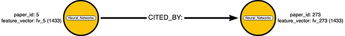
The papers were selected in a way such that every paper cites or is cited by at least one other paper. There are 2708 papers in the whole corpus and there are 5429 edges.
The Cora dataset forms part of the DGL data API and in order to make the workflow easy to replicate we have also used this version of the Cora set, which we will write as a graph in Neo4j. The only difference with the original Cora dataset is the node labeling, which is index-based in the DGL version.
However, there seem to be some duplicates, as DGL does filter them out with 5278 unique edges. Indeed when loading the Cora edges into Neo4j we also end up with 5278 relationships. Hence, the dataset has 5278 relationships, which we have termed as a ‘CITED_BY’ relationship type in Neo4j. We write the Cora graph to Neo4j, using the Python driver, as follows:
An excellent reference on how to use the Neo4j Python driver can be found in this article by Clair Sullivan.
Feature vectors
The text of each paper is analyzed and provides the feature vector as follows: after stemming and removing stopwords as well as words with a frequency of less than 10, we end up with 1433 unique words, which provides the dictionary. This dictionary now allows for the creation of a binary-valued feature vector (i.e. if the word appears in the document the vector entry is a 1, 0 otherwise), also known as a ‘bag-of-words’ representation. Hence, each document, representing a node in our case, has such a feature vector of length 1433.
The Task
We set the GAT to model a transductive learning task (semi-supervised learning) which is to predict the labels of the nodes but only allowing 20 nodes per class to be used for training, that is 140 out of a total of 2708. The training algorithm however is given the complete set of all nodes’ feature vectors. The trained model, again with only 140 training labels, is validated on 500 nodes and is tested on a set of 1000 nodes. This task can be applied to various real-world applications, for instance product labeling where the feature vectors are derived from the product description or client classifications where the feature vectors could be made up of co-purchases etc.
Hyperparameter selection
The Colab notebook that accompanies this article can be found here and includes detailed comments per code block. The key points to note are that the model selects 8 attention heads and given the small training set and risk of overfitting, the model uses both L_2 regularizations as well as dropout (at p = 0.6) to reduce this risk. Finally, cross-entropy is used as loss function with ADAM SGD optimizer
Running the Graph Attention Model
As mentioned earlier, the Deep Graph Library is one of the most extensive and well-documented graph machine learning libraries and has the added advantage of being able to run on either PyTorch, TensorFlow or MXNet.
The core of any machine learning model is the layer, which is not different in the DGL library, hence, the dgl.nn package contains the implementations of the most commonly used GNN layers, which of course includes the GAT layer. Finally, the DGL & TensorFlow combination is designed to work entirely using GPU’s.
Workflow
The code is commented in the Colab notebook, and the workflow is quite straightforward.
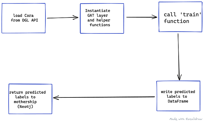
The data gets loaded into the notebook/model using the DGL data API and comes pre-processed using a mask method. This is a simple boolean vector either exposing or hiding the labels of the relevant train, validation, and test set. The GAT layer is a subclass of the TensorFlow-Keras layer where the arguments need to be determined when instantiating the class. To do this we created a separate function create_model, in addition to a few helper functions for the loss, accuracy, evaluate, early stopping etc.
Finally, the train function calls the relevant functions with its arguments determining the hyperparameters, which as listed above, we used the same as the paper.
We also made sure to write the predicted labels to a pandas DataFrame such that we can write them back to Neo4j.
As for training we selected 500 epochs but include an early stopping where we set the ‘patience’ at 100.
The running of the model takes less than 10 seconds and reaches the early stopping trigger after 379 epochs, achieving an impressive accuracy of 82.10%.
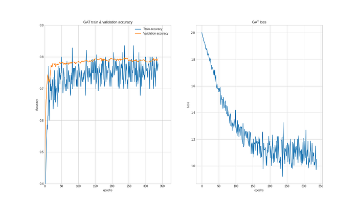
Thankfully, this is in line with the results achieved in the paper: 83.0% with a variance of 0.7%.
Hence, of the 1000 nodes in our test set the Graph Attention Network model managed to label 820 correctly, with only needing around 5% of the labels to train (140 out of 2708), and of course the features of every node.
Writing the Predicted labels to Neo4j
Now that our joint-venture with DGL has produced the results we needed, it’s time to head back to the mothership. Again, we call onto the Neo4j Python driver to write back the results to our Cora graph in Neo4j. This only takes us 7 lines of code plus the standard Cypher query, as follows:
We let the model run predictions on the entire graph, all 2708 nodes, and as can be seen from the Cypher query here above, we wrote the predicted labels to the graph as a node property.
We now have the following in Neo4j:
╒══════════════════════════════════════╕
│"n"                                   │
╞══════════════════════════════════════╡
│{"id":0,"label":"Genetic_Algorithms","│
│Predicted_Label":"Genetic_Algorithms"}│
├──────────────────────────────────────┤
│{"id":1,"label":"Rule_Learning","Predi│
│cted_Label":"Rule_Learning"}          │
├──────────────────────────────────────┤
│{"id":2,"label":"Rule_Learning","Predi│
│cted_Label":"Rule_Learning"}          │
├──────────────────────────────────────┤
│{"id":3,"label":"Case_Based","Predicte│
│d_Label":"Case_Based"}                │
├──────────────────────────────────────┤
│{"id":4,"label":"Genetic_Algorithms","│
│Predicted_Label":"Genetic_Algorithms"}│
└──────────────────────────────────────┘
And we can now run some Cypher queries, for instance, we can check how many predicted labels are different from the actual ones:
Which returned 454 — hence, we have 454 out of 2708 labels that are incorrect, or 16.7%, so indeed 83.3% being correctly predicted, which after stripping out the 140 training labels is exactly the same as the results from the paper.
We can also do some more detailed analysis in Neo4j by assigning the command above to an accuracy property, and then compute the accuracy per class of paper, as follows:
╒══════════════════════════════════╤══════════════════╕
│"Label"                           │"Accuracy"        │
╞══════════════════════════════════╪══════════════════╡
│["Theory"]                        │0.9425837320574163│
├──────────────────────────────────┼──────────────────┤
│["Probabilistic_Methods"]         │0.8986175115207373│
├──────────────────────────────────┼──────────────────┤
│["Rule_Learning"]                 │0.8943661971830986│
├──────────────────────────────────┼──────────────────┤
│["Case_Based"]                    │0.8062678062678063│
├──────────────────────────────────┼──────────────────┤
│["Reinforcement_Learning"]        │0.738255033557047 │
├──────────────────────────────────┼──────────────────┤
│["Genetic_Algorithms"]            │0.7286063569682152│
├──────────────────────────────────┼──────────────────┤
│["Neural_Networks"]               │0.7111111111111111│
└──────────────────────────────────┴──────────────────┘
Conclusion
In this article we have shown that by making use of the Neo4j Python driver a whole range of additional machine learning models can be accessed and complement the existing Neo4j GDS functionality.
In future articles we will illustrate how many of the Neo4j GDS algorithms can be used to compute a range of feature vectors which subsequently can be deployed to train a GNN, and again return the results to the native Neo4j graph.
